Probabilistic Source Code Modeling
How do we model the likelihood of code tokens in a sequence? This module covers n-gram language models, probability estimation, perplexity, smoothing, and why code is surprisingly predictable.
Probability Refresher
A quick recap of the probability concepts you will need throughout this module.
The sample space (S) is the set of all possible outcomes. For example, rolling a die gives S = {1, 2, 3, 4, 5, 6}. An event A = “roll an even number” = {2, 4, 6}, so P(A) = 3/6 = 0.5.
Conditional Probability
Example: A bag has 3 red and 2 blue marbles. You draw one and it is red (event B). What is the probability the next draw is also red (event A)? Since one red was removed, P(A|B) = 2/4 = 0.5.
The Chain Rule
To estimate the probability of an entire sentence, we need two building blocks: conditional probability and the chain rule.
From conditional probability we get the joint probability: P(A, B) = P(A) · P(B|A). For a sentence s = (w₁, w₂, …, wₙ), the chain rule expands this to:
Walkthrough: “its water is so transparent”
Applying the chain rule step by step:
- P(its)
- × P(water | its)
- × P(is | its water)
- × P(so | its water is)
- × P(transparent | its water is so)
The problem: to compute P(the | its water is so transparent that), we need Count(“its water is so transparent that the”) / Count(“its water is so transparent that”). Finding exact long sequences in any corpus is extremely unlikely — even huge corpora will never contain most long word sequences.
Maximum Likelihood Estimation
When we estimate probabilities by counting, we are using Maximum Likelihood Estimation (MLE) — the simplest and most intuitive way to learn a language model. Count occurrences, divide by total observations, and that is your probability estimate.
Worked Example
In a Java corpus, suppose Count(“(”, “for”) = 100 and Count(“(”) = 500. Then:
PMLE(“for” | “(”) = 100 / 500 = 0.20
The Data Sparsity Problem
To compute exact sequence probabilities, we would need enough data to observe every possible word combination. But the number of combinations is astronomical.
With just 1,000 unique words, the number of possible 5-word combinations is C(1000, 5) = 8.25 × 10¹². No corpus is large enough to observe all of these.
The solution: instead of conditioning on the entire history, approximate by conditioning on only the last few words. This is the Markov assumption, and it gives us n-gram models.
N-gram Models & the Markov Assumption
The key idea: approximate the full conditional probability by looking at only the last N−1 tokens.
| Model | Approximation |
|---|---|
| Unigram | P(w₁…wₙ) ≈ Π P(wᵢ) — each word independent |
| Bigram | P(wᵢ | w₁…wᵢ₋₁) ≈ P(wᵢ | wᵢ₋₁) — previous word only |
| Trigram | P(wᵢ | w₁…wᵢ₋₁) ≈ P(wᵢ | wᵢ₋₂, wᵢ₋₁) |
| N-gram | Condition on the last N−1 tokens. Higher N = more context but exponentially more data needed. |
Start & End Tokens
Language models need to know where sequences begin and end. Special boundary tokens <s> and </s> make this possible. Without <s>, the model cannot learn which tokens start sequences. Without </s>, the model cannot learn when to stop generating.
From <s> int x = 5 ; </s>, the resulting bigram pairs are:
Zipf’s Law & the Naturalness of Software
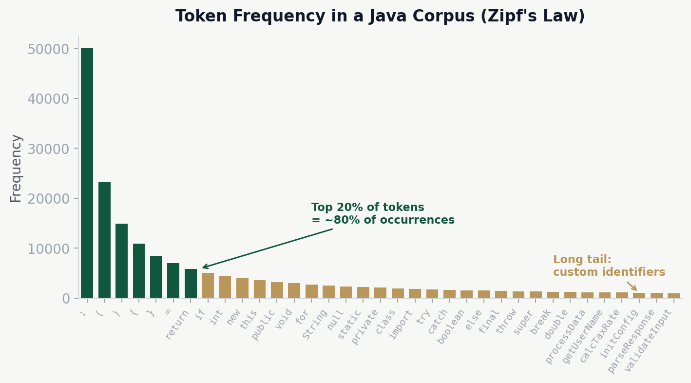
Word frequencies in natural language (and code) follow a power-law distribution known as Zipf’s Law: a small number of words occur very frequently, while a large number occur rarely. About 20% of words account for 80% of all occurrences.
In code, tokens like ;, =, (, ), return, if dominate, while most custom identifiers like processUserData or calcTaxRate fall in the long tail.
The Naturalness Hypothesis
Hindle et al. (ICSE 2012) made a groundbreaking discovery: “Programming languages, in theory, are complex and flexible, but real programs are mostly simple and rather repetitive, and thus they have usefully predictable statistical properties that can be captured in statistical language models.”
Both natural language and source code follow statistical patterns and have repetitive structures. But code is constrained by strict syntax rules and coding conventions, making it even more predictable than English.
The Naturalness Hypothesis
The theoretical foundation for applying language models to source code is the naturalness hypothesis, articulated by Hindle et al. at ICSE 2012. Their key finding was surprising: despite the theoretical expressiveness of programming languages, the code that developers actually write is highly repetitive and statistically predictable — in many cases more so than English prose.
The Key Experiment
Hindle et al. trained n-gram models on both English text (the Brown corpus and the Gutenberg corpus) and Java source code (a large open-source corpus). They measured cross-entropy on held-out test data and found a striking result:
Lower cross-entropy means higher predictability. The n-gram model was substantially less “surprised” by Java code than by English text. This means that at each token position, the model had fewer plausible next tokens to choose from when processing code.
Why Is Code More Predictable?
Several factors contribute to the naturalness of software:
- Strict syntax rules: programming languages enforce rigid grammatical structure. After
for (, only a handful of tokens are valid (int,var,;, an identifier), whereas English allows far more flexibility after any two-word prefix. - Coding conventions: style guides, naming conventions, and project norms reduce variability. Most Java developers write
for (int i = 0; i <rather than creatively varying loop syntax. - Repetitive idioms: common patterns like null checks, getter/setter methods, iterator loops, and try-catch blocks appear thousands of times across codebases with near-identical structure.
- API usage patterns: frameworks and libraries impose stereotyped call sequences. Using a
BufferedReaderalmost always follows the same open-read-close pattern. - Copy-paste culture: developers frequently reuse code snippets from documentation, Stack Overflow, or other parts of the same project, further increasing repetition.
Implications for Software Engineering
The naturalness hypothesis opened the door to an entire research area — applying statistical and machine learning techniques to source code. If code is predictable, then models trained on large code corpora can support practical tools:
Code Completion
Predict the next token or sequence of tokens as a developer types, reducing keystrokes and cognitive load.
Bug Detection
Flag code that has unusually low probability under the model — surprising code is often buggy code.
Code Review
Identify non-idiomatic patterns by detecting deviations from the statistical norm of the codebase.
Code Migration
Learn translation patterns between languages or API versions by exploiting statistical regularities in both source and target.
Training a Bigram Model
Training an n-gram model is simply counting. Split your corpus into training (80%) and test (20%) sets, count all bigram occurrences, then normalize each row to get probabilities.
Here’s what training an n-gram model looks like in practice — iterate through every token sequence, extract contexts, and count:
def train(self, methods, vocab):
    self.vocab = vocab
    self.vocab_size = len(vocab)
    for tokens in methods:
        p = pad(tokens, self.n)
        for i in range(self.n - 1, len(p)):
            for k in range(1, self.n + 1):
                ctx = tuple(p[i - k + 1 : i])
                self.counts[ctx][p[i]] += 1
                self.totals[ctx] += 1
In practice, a 3-way split is preferred: training (70%) for learning the counts, a held-out/validation set (10%) for tuning hyperparameters like interpolation weights λ, and a test set (20%) for final evaluation. The held-out corpus is specifically used for optimizing interpolation weights and smoothing parameters, and must be kept strictly separate from both training and test data — otherwise you risk overfitting your hyperparameters to the test set.
To prevent data leakage, we split by repository — all methods from one repo go into the same pool:
REPO_SPLITS = {
    "train": (1, 500),
    "val":   (501, 600),
    "test":  (601, 700),
}

def get_pool_name(rank):
    for pool_name, (lo, hi) in REPO_SPLITS.items():
        if lo <= rank <= hi:
            return pool_name
    return None
Simplified Count Matrix
| static | void | Inet4Address | ( | return | ip | |
|---|---|---|---|---|---|---|
| public | 120 | 15 | 8 | 5 | 2 | 0 |
| static | 0 | 180 | 45 | 3 | 0 | 0 |
| Inet4Address | 0 | 0 | 0 | 10 | 0 | 3 |
| if | 0 | 0 | 0 | 220 | 0 | 0 |
| return | 0 | 0 | 5 | 10 | 0 | 30 |
Example: P(getEmbeddedIPv4CA | Inet4Address) = Count(Inet4Address, getEmbeddedIPv4CA) / Count(Inet4Address) = 15 / 300 = 0.05
Worked Example: Building a Bigram Model
Let us walk through the entire process of building a bigram model from scratch, using a tiny Java corpus. This end-to-end example makes every step concrete: tokenization, counting, normalization, and prediction.
Step 1: The Corpus
Suppose our entire training corpus consists of three short Java statements:
int x = 0 ;
int y = x ;
return x ;
After adding boundary markers, our token sequences are:
<s> int x = 0 ; </s><s> int y = x ; </s><s> return x ; </s>
Step 2: Count All Bigrams
We scan every adjacent pair and tally the counts:
| Bigram | Count |
|---|---|
<s>, int | 2 |
<s>, return | 1 |
int, x | 1 |
int, y | 1 |
x, = | 1 |
y, = | 1 |
=, 0 | 1 |
=, x | 1 |
0, ; | 1 |
x, ; | 2 |
;, </s> | 3 |
return, x | 1 |
Step 3: Compute Conditional Probabilities
For each context token, divide each bigram count by the total count of that context. For example, the context <s> appears 3 times total (2 followed by int, 1 followed by return):
- P(int | <s>) = 2/3 = 0.667
- P(return | <s>) = 1/3 = 0.333
The context int appears 2 times (once before x, once before y):
- P(x | int) = 1/2 = 0.500
- P(y | int) = 1/2 = 0.500
The context = appears 2 times (once before 0, once before x):
- P(0 | =) = 1/2 = 0.500
- P(x | =) = 1/2 = 0.500
And ; always leads to </s>: P(</s> | ;) = 3/3 = 1.000.
Step 4: Use the Model to Predict
Given the partial input <s> int, what does our model predict next? We look up the distribution P(? | int):
The model assigns equal probability to x and y. With greedy decoding, we could pick either; with sampling, each has a 50% chance. Notice that any other token has probability zero under raw MLE — the model has never seen int followed by anything else. This illustrates the zero-count problem on even a tiny corpus.
Step 5: Score a Full Sequence
What is P(<s> int x = 0 ; </s>) under our bigram model?
P(int|<s>) × P(x|int) × P(=|x) × P(0|=) × P(;|0) × P(</s>|;)
= 0.667 × 0.500 × 0.500 × 0.500 × 1.000 × 1.000
= 0.0833
Pros & Cons of N-gram Models
Strengths
- No GPU needed — CPU computation is sufficient
- Easy to implement — just counting and dividing
- Fast to train and query
- Interpretable — inspect count tables directly
- Well-understood mathematical foundations
Limitations
- Cannot capture long-distance relationships
- Fixed context window (cannot see beyond N−1 tokens)
- Data sparsity grows exponentially with N
- No semantic understanding of tokens
- Cannot generalize to unseen n-grams
The long-range dependency problem: consider a variable ip1 declared at the top of a method but used many lines later in the return statement. A bigram or trigram model would have no knowledge of ip1 when predicting the final return — the declaration is far beyond its context window.
Evaluation: Perplexity & Cross-Entropy
Extrinsic evaluation tests a model on a downstream task (code completion, bug detection) and measures accuracy. It is the gold standard but expensive and time-consuming.
Intrinsic evaluation uses perplexity — a measure of model quality independent of any application. Lower perplexity = better model (less “surprised” by the test data).
Worked Example
Sequence: for ( int i (4 tokens)
- P(for | <s>) = 0.15
- P( ( | for ) = 0.85
- P( int | ( ) = 0.40
- P( i | int ) = 0.30
Product: 0.15 × 0.85 × 0.40 × 0.30 = 0.0153. Cross-entropy H = 1.508 bits. Perplexity = 21.508 = 2.84 — the model is as uncertain as choosing between ~3 equally likely next tokens.
In code, perplexity is computed in log-space to avoid floating-point underflow from multiplying many small probabilities:
def perplexity(self, methods):
    log_prob, n_tok = 0.0, 0
    for tokens in methods:
        p = pad(tokens, self.n)
        for i in range(self.n - 1, len(p)):
            ctx = tuple(p[i - self.n + 1 : i])
            log_prob += math.log2(self.prob(p[i], ctx))
            n_tok += 1
    return 2.0 ** (-(log_prob / n_tok)) if n_tok else float("inf")
Cross-Entropy
Perplexity Calculation Walkthrough
Let us take the bigram model we built in the worked example and compute perplexity on a test sentence, step by step. This makes every probability lookup and arithmetic operation explicit.
The Test Sentence
We want to evaluate our bigram model on the unseen sequence:
<s> int x = 0 ; </s>
This gives us N = 6 bigram transitions to evaluate (from <s> through </s>).
Step 1: Look Up Every Bigram Probability
Using the conditional probabilities we computed from the training corpus:
| Position | Bigram | P(wᵢ | wᵢ₋₁) | log₂ P |
|---|---|---|---|
| 1 | <s> → int | 2/3 = 0.6667 | −0.585 |
| 2 | int → x | 1/2 = 0.5000 | −1.000 |
| 3 | x → = | 1/3 = 0.3333 | −1.585 |
| 4 | = → 0 | 1/2 = 0.5000 | −1.000 |
| 5 | 0 → ; | 1/1 = 1.0000 | 0.000 |
| 6 | ; → </s> | 3/3 = 1.0000 | 0.000 |
Step 2: Sum the Log Probabilities
Working in log-space prevents floating-point underflow:
Σ log₂ P = (−0.585) + (−1.000) + (−1.585) + (−1.000) + 0.000 + 0.000
= −4.170
Step 3: Compute Cross-Entropy
Cross-entropy is the negative average of the log probabilities:
H = −(1/N) × Σ log₂ P = −(−4.170) / 6 = 0.695 bits
Step 4: Compute Perplexity
Perplexity is 2 raised to the cross-entropy:
PP = 2H = 20.695 = 1.62
Interpreting the Result
A perplexity of 1.62 is very low — the model is almost never surprised by this test sentence. This makes sense: the sentence int x = 0 ; appeared verbatim in the training data. The model has seen every bigram before, and several transitions (like 0 → ; and ; → </s>) have probability 1.0, contributing zero uncertainty.
In practice, perplexity on held-out test data is always higher than on training data. Typical values for well-trained code models range from 5 to 50, depending on the model order, corpus size, and vocabulary.
Smoothing: Handling Zero Counts
If count(wᵢ₋₁, wᵢ) = 0, then P(wᵢ|wᵢ₋₁) = 0. A single zero probability makes the entire sequence probability zero and perplexity infinite.
Laplace (Add-1) Smoothing
where V = vocabulary size. Simple but crude — steals too much mass from observed events.
| Bigram | Raw Count | +1 Count | Raw P | Smoothed P |
|---|---|---|---|---|
for ( | 18 | 19 | 18/100 = 0.180 | 19/110 = 0.173 |
for return | 0 | 1 | 0/100 = 0.000 | 1/110 = 0.009 |
Assumes count(for) = 100, V = 10
Add-k Smoothing
Generalize Laplace by adding k instead of 1. k is a hyperparameter — optimize it on a held-out set. Laplace is too crude for large vocabularies because it adds 1 to every possible bigram, redistributing enormous mass to unseen events.
The add-k formula translates directly into a single line of Python:
def prob_additive(self, token, ctx):
    return (self.counts.get(ctx, {}).get(token, 0) + self.alpha) / \
           (self.totals.get(ctx, 0) + self.alpha * self.vocab_size)
Smoothing Techniques Compared
Different smoothing methods handle the zero-count problem in different ways. Let us compare the three most important approaches using the same unseen bigram, so you can see exactly how each one redistributes probability mass.
Setup
Suppose our vocabulary has V = 1,000 tokens. The context token return appeared 200 times in training. The bigram return newList was never observed (count = 0). Meanwhile, the bigram return null was observed 80 times.
Comparison Grid
| Method | P(newList | return) (unseen bigram) | P(null | return) (seen bigram) | Key Trade-off |
|---|---|---|---|
| MLE (no smoothing) | 0 / 200 = 0.0000 | 80 / 200 = 0.4000 | Unseen events get zero — breaks perplexity |
| Laplace (add-1) | (0+1) / (200+1000) = 0.000833 | (80+1) / (200+1000) = 0.0675 | Steals too much mass — null drops from 0.40 to 0.07 |
| Add-k (k=0.01) | (0+0.01) / (200+10) = 0.0000476 | (80+0.01) / (200+10) = 0.3810 | Better balance — small mass to unseen, preserves observed |
| Kneser-Ney | Backed by continuation probability: ∼0.0003 | Count minus discount d: ∼0.3950 | Best overall — uses context diversity, not raw frequency |
Why Laplace Fails at Scale
The numbers above make the problem clear. With V = 1,000, Laplace adds 1 to every possible bigram count and adds V = 1,000 to the denominator. The observed bigram return null drops from probability 0.40 to 0.07 — an 83% reduction. Meanwhile, each of the ~920 never-seen bigrams after return receives probability 0.000833. In total, these unseen events steal the majority of the probability mass from events we actually observed.
Kneser-Ney: The Gold Standard
Kneser-Ney smoothing goes beyond simple count adjustment. Instead of asking “how often did w appear after this context?”, it asks “how many different contexts does w appear in?” This is called the continuation probability.
The intuition: a token like Francisco has a high raw unigram count (because it appears many times in “San Francisco”), but it only ever follows one context (San). Its continuation probability is low, reflecting that it is not a versatile word. In contrast, null follows many different contexts (return, =, !=, ==), so its continuation probability is high.
where d is a fixed discount (typically 0.75) and λ is a normalizing weight that distributes the discounted mass.
Interpolation & Backoff
Instead of relying on a single n-gram order, blend multiple models together for more robust probability estimates.
Linear Interpolation
where λ₁ + λ₂ + λ₃ = 1. Choose weights using a held-out validation set.
Worked Example
Predict next token after for ( with λ₁=0.1, λ₂=0.3, λ₃=0.6:
- Puni(int) = 0.05
- Pbi(int | () = 0.40
- Ptri(int | for, () = 0.65
P(int) = 0.1(0.05) + 0.3(0.40) + 0.6(0.65) = 0.005 + 0.12 + 0.39 = 0.515
Interpolation blends all sub-orders from unigram through n-gram, each weighted equally by 1/n:
def prob_interpolation(self, token, ctx):
    lam = 1.0 / self.n
    p = 0.0
    for k in range(1, self.n + 1):
        sub_ctx = ctx[-(k-1):] if k > 1 else ()
        c = self.counts.get(sub_ctx, {}).get(token, 0)
        t = self.totals.get(sub_ctx, 0)
        p += lam * (c + self.alpha) / (t + self.alpha * self.vocab_size)
    return p
Stupid Backoff
If the n-gram count is zero, back off to the (n−1)-gram: try trigram → bigram → unigram.
The formal definition from Brants et al.:
Because we back off without proper renormalization, this is not strictly a probability distribution — but it works well in practice at scale. Brants et al. found λ = 0.4 works well across many tasks.
Temperature & Sampling
Always picking the most likely next token (greedy decoding) produces repetitive, boring output. Sampling introduces variety by choosing randomly according to the probability distribution.
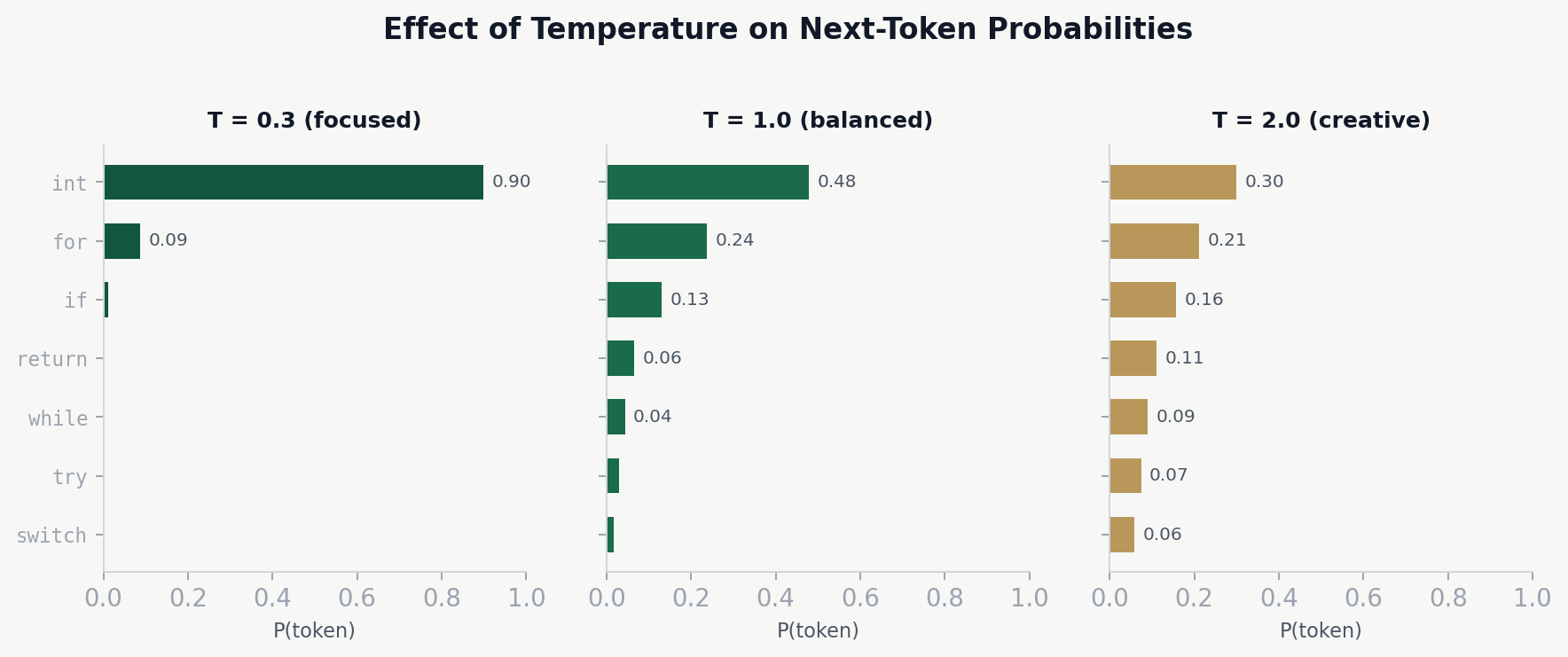
Temperature (T) controls the sharpness of the distribution:
- T = 0 (greedy) — always pick the highest-probability token
- T = 1 — sample from the actual learned distribution
- T > 1 — flatten the distribution — more random/creative
- T < 1 — sharpen the distribution — more focused/deterministic
Top-k sampling: only consider the k most probable tokens, discard the rest and renormalize.
Top-p / nucleus sampling: choose the smallest set of tokens whose cumulative probability exceeds p (e.g., p=0.9). Adapts to the shape of the distribution — keeps fewer tokens when the model is confident.
Concrete Example: Temperature in Action
Suppose our model has just processed the context return new and the raw logits (unnormalized scores) for the top five candidate tokens are:
| Token | Raw logit | T = 0.3 (focused) | T = 1.0 (neutral) | T = 2.0 (creative) |
|---|---|---|---|---|
ArrayList | 5.0 | 0.876 | 0.437 | 0.288 |
HashMap | 3.5 | 0.101 | 0.263 | 0.241 |
String | 2.0 | 0.012 | 0.142 | 0.197 |
Object | 1.5 | 0.006 | 0.105 | 0.175 |
int | 1.0 | 0.003 | 0.053 | 0.099 |
The temperature-scaled softmax formula divides each logit by T before applying softmax:
Reading across the table:
- T = 0.3:
ArrayListdominates with 87.6% probability. The model is almost certain — this is nearly greedy decoding. Useful for code completion where correctness matters more than variety. - T = 1.0: the original learned distribution.
ArrayListis still the top choice at 43.7%, but alternatives have meaningful probability. A reasonable default. - T = 2.0: the distribution is nearly flat. Even
int(the least likely candidate) has a 9.9% chance. This produces diverse but potentially incorrect or surprising output.
Out-of-Vocabulary & the <UNK> Token
New code uses identifiers not in training data: myCustomHandler, calcNetRevenue. These have zero probability.
Solution: replace rare tokens (count < threshold) with a special <UNK> token before training. The model learns “rare token behavior” — what typically follows or precedes an uncommon identifier. At test time, any unseen token maps to <UNK> and gets a nonzero probability.
The tradeoff: threshold too high loses valuable information; too low keeps sparsity. Finding the right balance requires experimentation.
Modern solution: this is why modern LLMs use BPE (Byte Pair Encoding) instead of word-level tokenization. BPE breaks words into subword units, so even unseen identifiers can be represented as sequences of known subwords — connecting back to the tokenization concepts from Module 1.
Building a vocabulary from training data and mapping unseen tokens to UNK at test time:
def build_vocabulary(methods):
    vocab = set()
    for m in methods:
        tokens = m['tokenized_code'].split()
        vocab.update(tokens)
    return vocab

def apply_unk(methods, vocab):
    result = []
    for m in methods:
        tokens = m['tokenized_code'].split()
        new_tokens = []
        for t in tokens:
            if t in vocab:
                new_tokens.append(t)
            else:
                new_tokens.append('<UNK>')
        result.append(' '.join(new_tokens))
    return result
From N-grams to Neural Language Models
N-gram models have two fundamental limitations that neural language models overcome:
- Parameter explosion: the number of parameters grows exponentially with the n-gram order. A 5-gram model with vocabulary V requires up to V⁵ parameters — quickly intractable.
- No generalization: n-gram models cannot transfer knowledge between similar contexts. Seeing “the cat sat” teaches nothing about “the dog sat” because the model treats every word as an independent symbol.
N-gram LMs
- Count-based statistics
- Fixed context window
- No semantic understanding
- Cannot generalize
- Fast, interpretable
Neural LMs
- Learned representations
- Long-range context
- Semantic embeddings
- Generalizes to new data
- GPU-intensive, less interpretable
Why N-grams Hit a Ceiling
Despite their elegance, n-gram models face three hard limits that no amount of data or smoothing can fully overcome:
- Sparsity is exponential: a bigram model with vocabulary V has V² possible entries; a 5-gram model has V⁵. For a modest code vocabulary of 50,000 tokens, a 5-gram table would need 50,000⁵ ≈ 3.1 × 10²³ cells — most of which will be zero regardless of corpus size.
- Fixed context is blind: an n-gram model with n = 5 cannot see the variable declared 20 tokens ago, the function signature 50 tokens ago, or the import statement 200 tokens ago. Code dependencies routinely span these distances.
- No shared representations: to an n-gram model,
ArrayListandLinkedListare completely unrelated symbols. Seeingreturn new ArrayLista thousand times teaches the model nothing aboutreturn new LinkedList— it must learn each combination independently from scratch.
How Neural Models Overcome These Limits
Each generation of neural architecture addressed a specific n-gram weakness:
Feed-Forward Neural LMs (Bengio, 2003)
Replace the sparse count table with a dense neural network. Each word is mapped to a continuous embedding vector, so similar words (e.g., ArrayList and LinkedList) share nearby representations. Solves the generalization problem, but still uses a fixed context window.
Recurrent Neural Networks
Process tokens one at a time, maintaining a hidden state that accumulates information from all previous tokens. In theory, the context window is unlimited. In practice, vanilla RNNs struggle with long-range dependencies due to vanishing gradients; LSTMs and GRUs partially address this.
Transformers (Vaswani et al., 2017)
Use self-attention to let every token attend directly to every other token in the sequence, regardless of distance. No recurrence needed — attention computes pairwise relevance in parallel. This solves both the fixed-window problem and the vanishing gradient problem.
Large Language Models
Scale transformers to billions of parameters, trained on trillions of tokens of code and text. Models like Codex, CodeLlama, and GPT-4 achieve perplexities that dwarf what any n-gram model can reach, and they can generate entire functions from natural language descriptions.
What Carries Forward
Despite these advances, the concepts from this module remain foundational. Neural language models still estimate P(next token | context) — the same conditional probability we have been computing. They are still evaluated using perplexity and cross-entropy. They still use temperature and top-k/top-p sampling for generation. And the naturalness hypothesis still explains why these models work so well on code.
Try It Yourself
Assignment: Recommending Code Tokens via N-gram Models
Build an n-gram language model for Java code completion. Train models for n ∈ {3, 5, 7}, implement smoothing to handle unseen n-grams, and evaluate using perplexity.
- Mine and prepare Java method-level data (replicate the MSR pipeline from Module 1)
- Create three nested training sets (T1 ≤ 15K, T2 ≤ 25K, T3 ≤ 35K), plus validation (~1K) and test (~1K) sets
- Build a separate vocabulary for each training set, map unseen tokens to
<UNK> - Train n-gram models for n ∈ {3, 5, 7} with smoothing (add-α or interpolation)
- Select the best configuration using validation perplexity
- Evaluate on both a provided test set and a self-created test set
Open the Exercise in Google Colab →
Code examples in this module are adapted from an implementation by Walker Hyman, an undergraduate student in Generative AI for Software Development at William & Mary.